AbsPipe formulation:
The formulation incorporates the 1D mass, energy and momentum equations in transient regime. The number of volumes in which the pipe is discretized is a parameter (nodes).
Numerical scheme
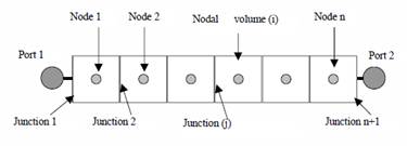
Pressures and temperatures are associated with the n nodes. The dynamic mass flows are calculated at the internal junctions (centred scheme, where each junction has associated two half volume inertias).
The mass flows at the first and last junctions (1 and n+1) will be given by the inductive type components connected to the pipe. Note that the first and last half-nodal inertia are included in the junction.
�Mass conservation equation
![]()
where�
![]() �is the volume of the
node i,
�is the volume of the
node i, ![]() is the massflow and ρ is the density of the node.
is the massflow and ρ is the density of the node.
Energy conservation equation

where��
![]() �is the volume of the
node i,
�is the volume of the
node i, ![]() is the massflow and ρ is the density of the node, u is
the internal energy, h the enthalpy,
is the massflow and ρ is the density of the node, u is
the internal energy, h the enthalpy, ![]() �is the velocity of the
fluid,
�is the velocity of the
fluid, ![]() �the slope of the pipe
and g gravity.
�the slope of the pipe
and g gravity.
Momentum equation
The following momentum balance equation dynamically calculates the massflow in each junction:

where I is the inertia of the fluid, P is
the static pressure calculated by the volume connected to the junction, ![]() �is the dynamic
pressure calculated as function of the density and the velocity calculated by
the volume connected to the junction and
�is the dynamic
pressure calculated as function of the density and the velocity calculated by
the volume connected to the junction and![]() is the pressure loss due to friction of the half of the
volume next to the junction.
is the pressure loss due to friction of the half of the
volume next to the junction.
The equivalent distributed friction, Δξ (i), is calculated as follows:
![]()
Where K_add is an input data representing concentrated load losses to be distributed along the pipe. Function 'hdc_bend' calculates the bend pressure drop coefficient (see Annex 1). Function 'hdc_fric' calculates the friction factor including laminar and turbulent regimes (see Annex 1).
The term qn(i) accounts for pressure losses due to turbulence terms not directly calculated with a 1D approach (see R7, R8). This term also stabilizes numerically the system of equations. It is calculated as follows:
![]()
Where m_jun is the massflow in the corresponding junction and vsound is the speed of sound. A is the area of the cross section of the pipe.
Pressure, temperature and quality calculation
At each discretized volume, the non derivative state variables (pressures, qualities and temperatures) will be calculated using the state function:
CRYO_FL_state_vs_RU( f_in.fluid, f_in.eos, rho[i], u[i]-0.5*vel[i]**2, phase[i], rho_l[i], rho_g[i], P[i], T[i],Tsat[i], h_l[i], h_g[i], x[i], alpha[i], cp[i], cp_l[i], cp_g[i],drho_dp[i],drho_dh[i],vsound[i], visc[i], visc_l[i], visc_g[i], cond[i], cond_l[i], cond_g[i], sigma[i], ier[i] )
The sonic flow per unit of area is calculated at each pipe port as a function of the corresponding node pressure, density and the sound speed. These critical flows will be used at the connected inductive type components to take into account sonic flow limitation.